To interact with this Notebook: . To download this Notebook: click here.

First Application

This notebook introduces basic Coba functionality for contextual bandit application research. That is, evaluating how learners perform in specific environments.

Creating Environments

The primary means of performing application research in coba is to create coba environments that emulate the desired application.

The easiest way to do this is with domain specific datasets. Here we discuss three types of datasets that can be used.

1. Supervised Datasets

Perhaps the easiest way to get started is with domain relevant supervised datasets.

These kind of datasets can be generated in lab based validation studies that provide ground truth data that may not be available at deployment time. While these datasets may be unrealistic in a deployment scenario they can still indicate the feasiblility of using contextual bandit learners. Use cb.Environments.from_supervised, as shown below, to ingest labeled features as a coba environment.

import coba as cb

X = [[1,2,3],[4,5,6],[7,8,9]]    #these are features
Y = ['label1','label2','label3'] #these are class labels

cb.Environments.from_supervised(X,Y,label_type='c')

1. {'source': '[X,Y]', 'label_type': 'c', 'env_type': 'SupervisedSimulation'} | BatchSafe(Finalize())

2. Explicit Datasets

If you have a good model or understanding of your domain you might want to create an environment from scratch.

This can be done by implementing the environments interface (This could also be done using dataframes with appropriate column names).

import coba as cb

class MyEnvironment:

    def read(self):
        context = [[1,2,3,4], [4,5,6,7], [7,8,9,0]]
        actions = [['a','b'], ['a','c'], ['c','f']]
        rewards = [[1.2,0.1], [0.5,0.0], [0.3,5.0]]

        for C,A,R in zip(context,actions,rewards):
            yield {'context':C, 'actions': A, 'rewards': R }

list(cb.Environments.from_custom(MyEnvironment())[0].read())

[{'context': [1, 2, 3, 4],
  'actions': ['a', 'b'],
  'rewards': DiscreteReward([['a', 'b'], [1.2, 0.1]])},
 {'context': [4, 5, 6, 7],
  'actions': ['a', 'c'],
  'rewards': DiscreteReward([['a', 'c'], [0.5, 0]])},
 {'context': [7, 8, 9, 0],
  'actions': ['c', 'f'],
  'rewards': DiscreteReward([['c', 'f'], [0.3, 5]])}]

Logged Datasets

If you are working with an already deployed system there’s a good chance you will have logged bandit data.

Coba has many tools to work with this kind of data once it has been ingested.

The easiest way to ingest this data is to use dataframes.

import coba as cb
import pandas as pd

context     = [[1,2,3,4], [4,5,6,7], [7,8,9,0]]
action      = ['a', 'c', 'f']
reward      = [1.2, 0.0, 5.0]
probability = [0.1, 0.9, 0.2] #This is optional, but if you have it available coba can use it to improve certain estimators

df = pd.DataFrame({'context':context, 'action':action, 'reward':reward, 'probability': probability})

list(cb.Environments.from_dataframe(df)[0].read())

[{'context': [1, 2, 3, 4], 'action': 'a', 'reward': 1.2, 'probability': 0.1},
 {'context': [4, 5, 6, 7], 'action': 'c', 'reward': 0.0, 'probability': 0.9},
 {'context': [7, 8, 9, 0], 'action': 'f', 'reward': 5.0, 'probability': 0.2}]

Pre-processing Environments

Once you’ve created an environment you’d like to apply contextual bandit learners on it’s time to pre-process. Coba provides several convenience methods to prep your data for learning. In fact, you can even run experiments to see which pre-processing steps most improve CB learner performance. Below we demonstrate a few of these on synthetic data but you’d be working with an environment created using one of the methods described at the top of this notebook.

#scale applies centering and scaling to feature columns. You can even supply
#the 'using' argument to only scale based on a subset of the entire environment
cb.Environments.from_linear_synthetic(100).scale('med','iqr',using=100)

#impute fills in missing values (i.e., None values) with the chosen statistic
#by setting indicator=True an additional 1/0 feature is added to indicate to learners
#when a feature has been imputed
cb.Environments.from_linear_synthetic(100).impute('median',indicator=True)

#dense will apply the "hashing trick" to turn sparse data into dense representations
cb.Environments.from_linear_synthetic(100).dense(n_feats=2**10, method="hashing")

#noise will apply noise to context features, action features, or reward values
#noise is very useful to see how robust a learner would be to poor data at deployment
cb.Environments.from_linear_synthetic(100).noise(context=(0,.1),reward=(0,1))

#cycle can be used to check your robustness to non-stationarity. Cycle will wrap
#reward values to the right one space, which cycles the optimal action right as well.
cb.Environments.from_linear_synthetic(100).cycle(after=100)

#sort can be used to check your robustness to domain-shift. Sorting on context
#creates an environment where context distribution is a function of time step
cb.Environments.from_linear_synthetic(100).sort()

1. LinearSynth(A=5,c=5,a=5,R=['a', 'xa'],seed=1) | Sort('sort_keys': '*') | BatchSafe(Finalize())

Running Experiments

Once your environment has been prepped you are ready to run an experiment.

For this example we’re going to use an openml dataset, but everything we do below could be done with an environment you created.

Feature Scaling Experiment

#This shows how to evaluate what scaling logic works for your environment
env = cb.Environments.from_openml(180, take=4000)
env = env + env.scale('min','minmax',using=2000) + env.scale('mean','std',using=2000) + env.scale('med','iqr')
env = env.shuffle(n=10)

lrn = cb.VowpalEpsilonLearner()

cb.Experiment(env,lrn).run(quiet=True,processes=10).plot_learners(x=['shift','scale'], err='bs')

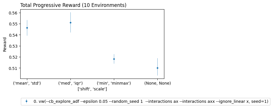
Above we see that for this environment either standardizing or robust scaling the context features seems to give the best performance.

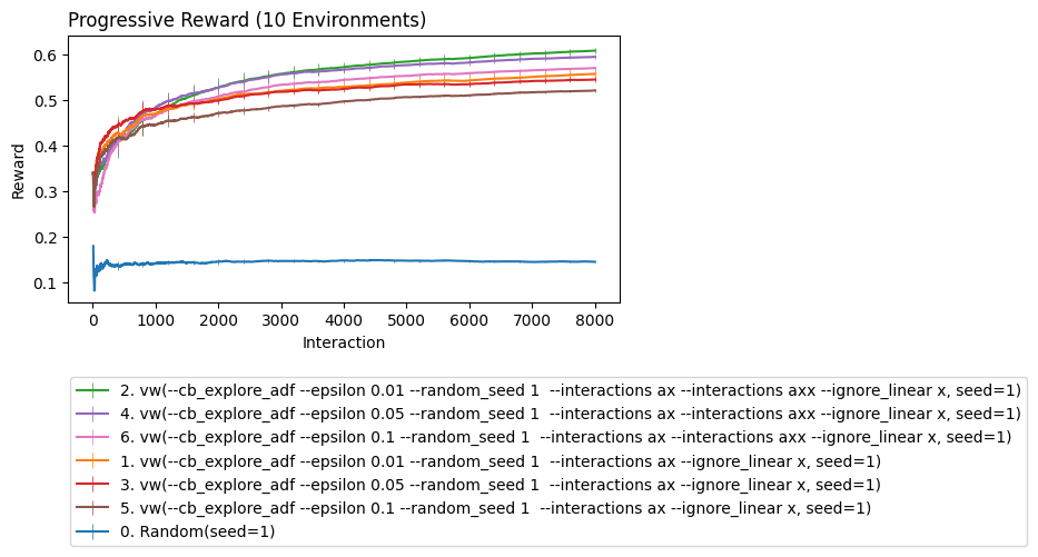
Hyperparameter Tuning

Coba doesn’t offer any out of the box methods like random search or halving.

Instead we rely primarily on experiment level paralellization to make explicit searches computationally viable.

The legend in coba plots will always be sorted according to learner performance to make it easier to pick out the best.

#This demonstrates how to do a hyperparameter sweep across VowpalEpsilonLearner

env = cb.Environments.from_openml(180, take=8000).scale('med','iqr').shuffle(n=10)

lrn = [cb.RandomLearner()]
for epsilon in [.01, .05, .1]:
    for feats in [(1,'a','ax'),(1,'a','ax','axx')]:
        lrn.append(cb.VowpalEpsilonLearner(epsilon=epsilon,features=feats))

cb.Experiment(env,lrn).run(quiet=True,processes=10).plot_learners(xlim=(10,None),err='bs')

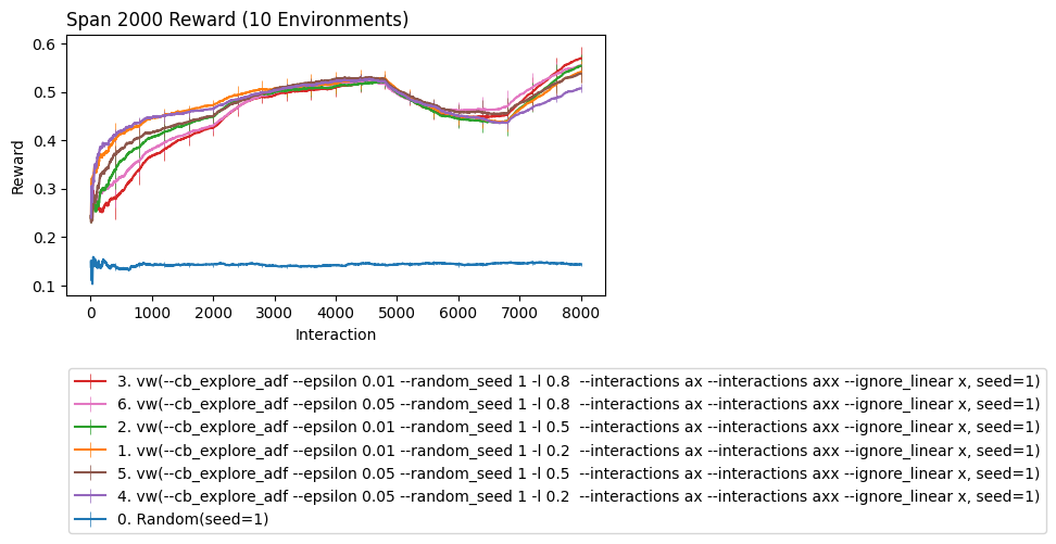
Robustness to Extreme Non-stationarity

The cycle shock we show below is an absolute worst case. Even so we see that our learner can be paramaterized in ways to be more robust.

#This demonstrates how to do a hyperparameter sweep across VowpalEpsilonLearner

env = cb.Environments.from_openml(180, take=8000).scale('med','iqr').shuffle(n=10).cycle(after=4000).riffle(6)

lrn = [cb.RandomLearner()]
for epsilon in [.01, .05]:
    for feats in [(1,'a','ax','axx')]:
        lrn.append(cb.VowpalEpsilonLearner(epsilon=epsilon,features=feats,l=.2))
        lrn.append(cb.VowpalEpsilonLearner(epsilon=epsilon,features=feats,l=.5))
        lrn.append(cb.VowpalEpsilonLearner(epsilon=epsilon,features=feats,l=.8))

cb.Experiment(env,lrn).run(quiet=True,processes=10).plot_learners(xlim=(10,None),err='bs',span=2000)

Running Experiments on Logged Data

Coba has considerable support for analysis using logged data. This is covered in detail in Logged Bandit Data.